
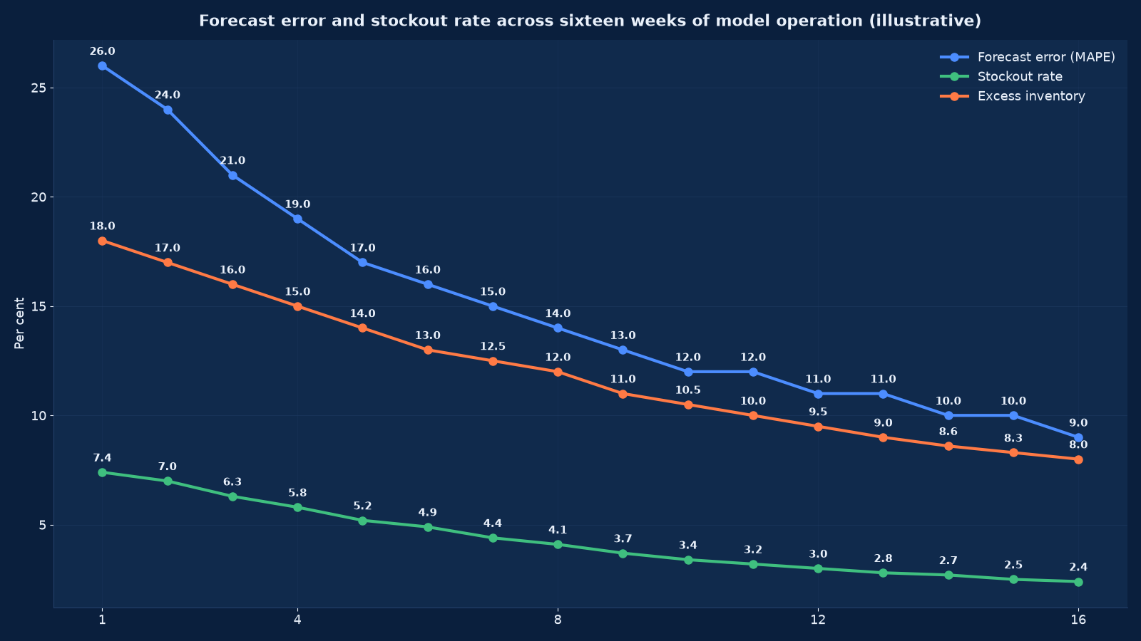
Chart values are an illustrative planning model based on typical UMC engagements and published industry benchmarks. They are not a guarantee of results on any specific project.
A forecast is not a prediction. It is an input to a decision — and its quality is measured by the cost of the decision it improved, not by how impressive the model was.
Predictive analytics and demand forecasting replaces judgement-only planning with a measured, monitored forecast at the grain your decisions are actually taken at — SKU by location by week, customer by month, machine by shift. Unified Management Consulting builds these against a naive baseline the model must beat, validated by walk-forward backtesting, deployed with monitoring and an owner, and connected to the ordering, staffing or pricing decision rather than delivered as a report.
🔮 Predictive Analytics & Demand Forecasting — Quick Summary
| Component | What We Deliver |
|---|---|
| Use case first | One decision with a measurable cost: inventory, stockouts, churn, credit, maintenance or capacity. If the decision cannot be named, the model cannot be justified. |
| Baseline discipline | Every model is compared against a naive baseline — last period, seasonal naive, moving average. A model that does not beat it is not deployed. |
| Grain and horizon | Declared before modelling: what is forecast, at what level of detail, how far ahead, and how often it is refreshed. |
| Feature engineering | Seasonality, promotions, price, weather, holidays, lead times, macro and lagged demand built from documented sources rather than scraped guesses. |
| Model selection | Statistical methods where data is thin and explainability matters; gradient-boosted or deep models where volume and complexity justify them. |
| Walk-forward validation | Backtested across many rolling origins, never a single split, so the error estimate reflects how the model will actually be used. |
| Uncertainty, not only a number | Prediction intervals published alongside the point forecast, because safety stock and staffing decisions are made on the range. |
| Decision integration | The forecast lands in the ordering, planning or staffing workflow with a named owner and an override reason captured. |
| Model operations | Drift monitoring, accuracy tracking, scheduled retraining, and a documented process for when the model is wrong in a way that matters. |
Prediction sits on the data platform described in our data warehouse service and on the governed measures from Data Science Services for Business Analytics. Where the consumer is a language model or an agent rather than a planner, Data Engineering for AI: RAG & Knowledge Systems and AI Product Engineering Services are the adjacent engagements. Where the question is whether the investment is worth making at all, AI ROI Measurement & Executive Scorecard Services supplies the scorecard.
Where Prediction Pays, and Where It Does Not
Predictive work fails most often at selection rather than at execution: a use case is chosen because it is interesting rather than because a costly decision sits behind it. Figure 2 ranks six use cases by the annualised value we typically observe in mid-market operations.
| Use case | The decision it improves | Data required | Typical payback |
|---|---|---|---|
| Demand forecasting for inventory | How much to buy, produce and hold at each location for each period | Two to three years of demand history at SKU-location-week grain, plus promotions, price, stockouts and lead times | Working capital release and lost-sales reduction usually repay the build inside two to four quarters |
| Customer churn prediction | Which accounts get retention attention this month, and with what offer | Usage, support tickets, payment behaviour, contract terms, engagement decay | Fast where retention cost is low relative to customer value; slow where churn is already rare |
| Credit and collection risk | Which customers get terms, what limit, and which invoices get chased first | Payment history, ageing, bureau data where available, order patterns, sector | Reduces bad debt and shortens collection cycles; the cash effect is immediate |
| Predictive maintenance | Which assets are serviced before failure rather than after | Sensor or meter readings, work-order history, failure records, operating conditions | Strong where failure is costly and data exists; weak where failures are rare and unlogged |
| Capacity and shift planning | How many people, machines or slots are needed per period | Volume history, service-level targets, shrinkage, absence, lead times for hiring | Reduces overtime and service breaches; effect visible within one planning cycle |
| Price and promotion response | What price and what depth of promotion, in which period, for which segment | Price and promotion history with volumes, competitor pricing where obtainable, elasticity variation | High value but requires genuine historical price variation, which most businesses lack |
| Sales and pipeline forecasting | What will close, when, with what probability | Deal history with stage timings, attributes and outcomes | Improves planning and capacity decisions; see our sales analytics service |
The three tests we apply before accepting a use case. Is there a decision that changes as a result, with a named owner? Is the cost of being wrong measurable in rupees? And does the data exist at the grain the decision needs — not approximately, but actually? A use case failing any of the three is deferred, and saying so is worth more than building it.
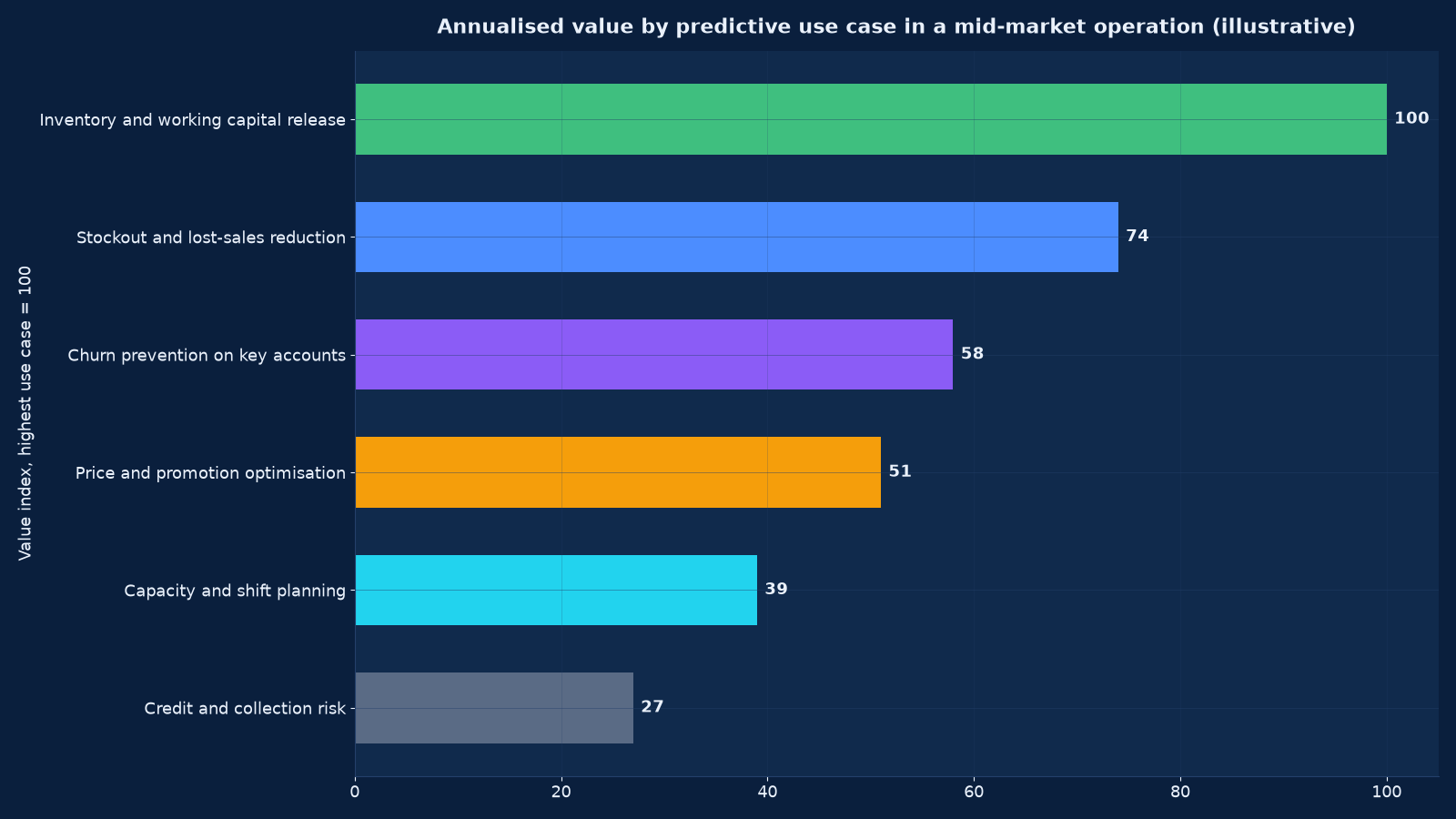
Chart values are an illustrative planning model based on typical UMC engagements and published industry benchmarks. They are not a guarantee of results on any specific project.
Model Selection: Why the Simple Model Usually Wins First
Method choice follows data volume, driver complexity and the need for explainability. In most mid-market engagements the winning model is exponential smoothing or gradient-boosted trees beating a seasonal naive baseline by a meaningful margin — not a deep architecture.
| Method | How it works | Choose it when | Do not choose it when |
|---|---|---|---|
| Seasonal naive | Forecast equals the same period last year | Always, as the baseline every other method must beat | Never as the answer once history and drivers exist |
| Exponential smoothing (ETS) | Weighted average of history with level, trend and seasonal components | Short history, stable patterns, one series at a time, explainability required | Many external drivers or thousands of interdependent series |
| ARIMA / SARIMA | Autoregressive and differenced moving-average model of the series itself | Clear autocorrelation structure and enough history to estimate it | Promotional or event-driven demand, where the drivers matter more than the history |
| Regression with drivers | Demand explained by price, promotion, weather, macro and calendar variables | You need to know why demand moves, and the drivers are measurable | Relationships are strongly non-linear or interactive |
| Gradient-boosted trees | Ensemble of trees over lagged demand, calendar and driver features | Many series, rich features, non-linear and interaction effects, and enough data to validate honestly | Thin data, or where a planner must be able to interrogate every term |
| Deep learning (temporal fusion, N-BEATS class) | Neural architectures learning shared structure across many series | Thousands of series, long history, and engineering capability to operate them | A mid-market business with two hundred SKUs — the accuracy gain will not repay the complexity |
| Hierarchical reconciliation | Forecasts made at several levels and reconciled so they sum consistently | SKU, category, region and group forecasts must all agree | Only one level is ever used, in which case it is unnecessary overhead |
The rule we apply. Start with the naive baseline, then the statistical model, then a feature-rich learner, and stop at the first method whose improvement over the previous one does not justify its complexity and operating cost. Publishing the comparison is part of the deliverable, because a business that has never seen its own baseline cannot tell whether a model is good. Our data science capability roadmap covers the skills required to operate each tier internally.
Demand Forecasting: Grain, Horizon and Refresh
A forecast is only useful at the grain where the decision is taken and over the horizon the decision covers. Declaring both before modelling is what prevents the common failure of an accurate monthly national forecast that cannot tell a plant what to make on Tuesday.
| Decision | Grain | Horizon | Refresh | What the forecast must include |
|---|---|---|---|---|
| Raw material purchasing | Item by supplier | 4–16 weeks, respecting lead time | Weekly | Point forecast, interval, and the lead-time distribution |
| Production scheduling | SKU by line by day | 1–6 weeks | Daily or weekly | Point forecast with the capacity constraint stated |
| Finished-goods replenishment | SKU by location by week | 2–13 weeks | Weekly | Point forecast, interval, and stock on hand and in transit |
| Distribution and inventory rebalancing | SKU by warehouse | 1–8 weeks | Weekly | Forecast per location plus the transfer cost and time |
| Workforce and shift planning | Team by day or shift | 2–12 weeks | Weekly | Volume forecast with the service-level target and shrinkage |
| Cash and working capital planning | Business unit by month | 3–13 months | Monthly | Revenue and cost forecast with the range, feeding the cash forecast |
| Promotion and pricing | SKU by promotion event | Event horizon plus post-event decay | Per event | Baseline, uplift, cannibalisation and post-promotion dip |
Hierarchy and reconciliation. Where forecasts exist at SKU, category, region and group levels, they must sum consistently. Reconciling them is a modelling decision with a direct consequence: an unreconciled set produces the familiar meeting where three accurate forecasts disagree and nobody can say which governs the decision.
Features: Where the Accuracy Actually Comes From
Model architecture contributes less to accuracy than feature quality. These are the feature families that matter, in the order we build them.
- Lagged demand and rolling statistics. Lags at one, two, four, thirteen, twenty-six and fifty-two periods; rolling means, medians and standard deviations. The single strongest family in almost every dataset.
- Calendar structure. Day of week, week of month, month, quarter, working days, pay cycles, and the festival and holiday calendar specific to your markets — including the fact that a festival’s date moves between years.
- Promotion and price. Depth, duration, mechanics, feature placement, competitor activity where known, and the post-promotion dip that most models miss.
- Availability and censoring. Stockout periods must be identified and demand estimated rather than recorded, because recorded sales during a stockout are zero and true demand is not. This correction alone frequently changes the answer more than the model choice.
- External drivers. Weather where the category is weather-sensitive, macro indicators, fuel and input prices, and sector-specific events.
- Product lifecycle and substitution. Launch, growth, decline, discontinuation and cannibalisation between variants — without which a new SKU forecast is meaningless and a discontinued one is over-forecast.
- Hierarchical and cross-series features. Category and group aggregates, which stabilise intermittent SKU-level series.
Intermittent demand needs its own treatment. Slow-moving and lumpy items — spare parts, capital goods, low-volume SKUs — violate the assumptions of standard error metrics and are better served by Croston-class methods or by explicit interval and service-level targets rather than a point forecast. Measuring them with the same accuracy metric as fast movers is how a forecasting programme ends up optimising the wrong half of the range.
Validation: Backtesting Done Properly
A single train-test split tells you almost nothing about a forecasting model. Four practices are non-negotiable.
Walk-forward evaluation across many origins. The model is re-estimated at rolling points in history and evaluated on the periods that followed each, so the error estimate reflects how the model will actually be used — repeatedly, on data it has not seen, with the future always ahead of it.
The naive baseline published alongside. Seasonal naive, last value and a moving average, on the same origins and the same metric. If the model does not beat all three, it is not deployed.
Metrics matched to the decision. MAPE flatters low-volume items and is undefined at zero; WMAPE or MAD scaled by volume is usually the honest choice for inventory. Where the cost of over-forecasting differs from under-forecasting — perishables, fashion, committed capacity — an asymmetric loss metric is used, because a symmetric metric will produce a symmetric answer to an asymmetric problem.
Residual and bias review. Systematic over- or under-forecasting in a segment, a season or a promotion type is a modelling defect, not noise. Bias is what erodes trust, and it is detected by reviewing residuals by segment rather than in aggregate.
Where the series is short or the domain is unusual, we say so and widen the interval rather than present a false precision. A forecast the planner does not trust is not used, and a forecast that is not used has no value however accurate it is.
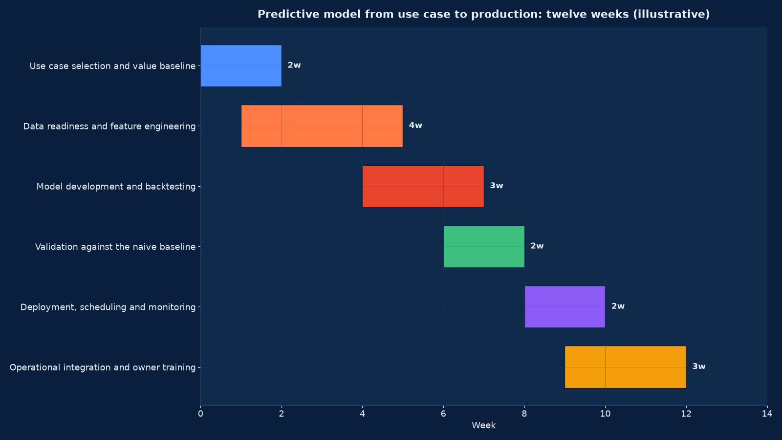
Chart values are an illustrative planning model based on typical UMC engagements and published industry benchmarks. They are not a guarantee of results on any specific project.
The Twelve-Week Programme
| Phase | Weeks | Activities | Output |
|---|---|---|---|
| Use case selection and value baseline | 1–2 | The decision named, its current cost measured, the improvement required to justify the build, and the owner identified | A one-page business case with a measurable baseline |
| Data readiness | 2–4 | History assembled at the required grain, stockouts and censoring identified, promotions and prices joined, gaps documented | A modelling dataset with a written data-quality statement |
| Feature engineering | 3–5 | Lags, calendar, promotion, availability, lifecycle and external features built and documented | A version-controlled feature pipeline |
| Baseline and model development | 5–7 | Naive and statistical baselines established, candidate models developed, hyperparameters tuned on validation folds only | A ranked set of candidates against a published baseline |
| Walk-forward validation | 7–8 | Rolling-origin backtesting, metric selection matched to the decision, bias and residual review by segment | An error estimate the business can rely on |
| Deployment and scheduling | 9–10 | Automated retraining and inference, output landed where the decision is taken, intervals published, failure alerting | A forecast produced without manual intervention |
| Operational integration and training | 10–12 | Override process with reason capture, planner training, monitoring dashboard, ownership handover | A working process with a named owner |
Model Operations: The Part That Determines Whether It Survives
Models decay. Demand patterns shift, promotions change character, a competitor enters, a supplier lead time lengthens, and a model validated in week eight is describing a market that no longer exists by month eighteen.
- Accuracy tracking against the live baseline. The naive baseline is re-computed every period alongside the model, so the model’s continuing advantage is visible rather than assumed.
- Drift monitoring. On input feature distributions and on forecast error by segment. A drift alert is a prompt to investigate, not an automatic retrain.
- Scheduled retraining with review. Automatic refresh of parameters on a fixed cadence, with structural re-specification reviewed annually or after a material change.
- Override governance. Planners may and should override, but every override carries a reason and is measured. Over time the override record shows whether the model or the planner is more accurate in which situations — which is the most valuable output of the whole operating process.
- Failure handling. What happens when the pipeline breaks, when a source is late, and when the forecast is materially wrong: fallback to the last good run, alert to a named owner, and a documented decision rule.
- Version control and reproducibility. Model code, features, parameters and training data versions retained so any published forecast can be reproduced and explained months later.
This is the same operate-don’t-demo discipline as AI Governance, Risk & Compliance applies to generative systems, and the same cost-control question Cloud Cost Optimisation & FinOps applies to the compute behind a continuously retrained model estate.
From Forecast to Decision
A forecast that is not connected to a decision is an expensive report. Four connections are designed explicitly.
Safety stock and service level. The prediction interval, not the point forecast, sets safety stock. A target service level per SKU class converts the interval into a reorder point, which is where the working capital release in Figure 2 actually comes from — better intervals allow lower stock at the same service level.
Sales and operations planning. The forecast enters a monthly S&OP cycle with a defined consensus process: statistical forecast, commercial input, supply constraint, agreed number, and a record of who changed what and why. Without that record the organisation learns nothing from being wrong.
Ordering and replenishment automation. Where the decision is routine, the forecast should generate a proposed order that a person approves rather than a number a person re-derives. The approval threshold is set from the forecast’s own error rate.
Financial planning. The demand forecast is the volume input to the revenue forecast, the production budget and the cash forecast. Where finance plans separately from operations, the business runs two forecasts and reconciles them by argument. Cash Flow & Working Capital Recovery is where the inventory release becomes liquidity, and the thirteen-week cash forecast there takes its volumes from here.
Measuring the Programme
The seventh row is the one we report to the owner, because it isolates what the model contributes over what the business could have done for free. A model with negative forecast value added in a segment is switched off in that segment.
| Measure | Definition | Target |
|---|---|---|
| Forecast error (WMAPE or MAD) | Volume-weighted absolute error against actuals at the decision grain | Beating the seasonal naive baseline by a clear margin, improving each quarter |
| Bias | Signed error, reviewed by segment and season | Near zero; systematic bias is treated as a defect |
| Interval coverage | Share of actuals falling inside the published prediction interval | Close to the nominal level — an interval that is wrong is worse than none |
| Stockout rate | Share of demand occasions not met from stock | Falling against baseline |
| Excess and slow-moving inventory | Value of stock above the service-level requirement, and stock with no movement in a defined period | Falling; the working capital release is measured here |
| Inventory turns | Cost of sales over average inventory | Rising |
| Forecast value added | Model error minus baseline error, per segment | Positive, and negative segments investigated or reverted to baseline |
| Override rate and override accuracy | Share of forecasts overridden and whether overrides improved the outcome | Falling override rate with overrides demonstrably better where they persist |
| Planning time saved | Hours per cycle spent assembling rather than deciding | Falling by half or more |
| Model uptime and freshness | Share of scheduled runs completing on time | Above 99% |
Running This in an Indian Mid-Market Business
Conditions that change the model rather than merely complicating it.
Festival-driven demand with moving dates. Diwali, Dussehra, regional new years, Raksha Bandhan, Eid, Christmas and wedding seasons shift between Gregorian weeks each year. Encoding them as festival-relative features rather than calendar-month effects is usually the single largest accuracy improvement available in Indian consumer and retail data.
Monsoon and agricultural cycles. For FMCG, agri-input, two-wheeler and rural distribution categories, rainfall and harvest timing move demand more than promotion does, and they enter as external features rather than as unexplained seasonality.
Stockout-censored history. Availability is frequently poor in the tail of the range, so recorded sales understate demand precisely where the model is most needed. Identifying and correcting censored periods is a prerequisite, not a refinement.
General trade and distributor data gaps. Where sell-out is not captured from retail outlets, only sell-in is visible, and forecasting sell-in without sell-out builds inventory rather than satisfying demand. A distributor stock reporting process is often a cheaper and faster improvement than a better model.
Thin history and rapid change. New SKUs, new cities and fast-changing channels mean short series. Hierarchical borrowing from category and comparable-item patterns, with wider intervals and explicit judgement in the first cycles, is the honest approach — and the reason we publish intervals rather than single numbers.
Where Predictive Programmes Fail
None of these are modelling failures. They are measurement, governance and selection failures — and every one of them is prevented by a decision taken in the first fortnight rather than by a better algorithm in week eight.
| Failure mode | How it presents | Prevention |
|---|---|---|
| No baseline | Accuracy is quoted as a single number with nothing to compare it to | The seasonal naive baseline is computed every period and published beside the model |
| A single train-test split | Reported error is far better than live error | Walk-forward evaluation across many rolling origins |
| Wrong metric for the decision | MAPE looks good while the items that matter are badly forecast | Volume-weighted error, and an asymmetric loss where over- and under-forecasting cost differently |
| Forecasting censored demand | The model learns that demand collapses whenever stock runs out | Stockout periods identified and demand estimated before modelling |
| Point forecasts only | Safety stock is set by rule of thumb and the interval is never used | Intervals published, calibrated, and connected to the service-level policy |
| No override record | Planners adjust numbers silently, so nobody learns who is right | Every override carries a reason and is measured against the outcome |
| Modelled once, never monitored | Accuracy decays over eighteen months and is discovered by a stock crisis | Drift and accuracy monitoring with alerting to a named owner |
| Unreconciled hierarchy | SKU, category and group forecasts disagree in the same meeting | Hierarchical reconciliation designed in, not patched afterwards |
| Intermittent items judged as fast movers | Spare parts show terrible accuracy and drag the programme’s reputation | Separate methods and metrics for lumpy demand, reported separately |
| No decision owner | A good forecast that changes nothing | The decision, its owner and the cost of being wrong are named in week one |
The tenth row is the one that kills programmes outright. A model with no decision owner is maintained by nobody, consulted by nobody and retired by nobody; it simply stops being right while still being produced, which is the most expensive possible outcome because it continues to cost money and continues to be quoted.
Engagement Models
| Model | Duration | Deliverables | Best when |
|---|---|---|---|
| Predictive feasibility assessment | 2–3 weeks | Use case ranking by value and feasibility, data readiness statement, baseline measurement and a recommended first model | You want prediction but do not know which decision to attack first |
| Demand forecasting build | 12 weeks | Feature pipeline, validated model with published baseline comparison, intervals, deployment, override governance and planner training | Inventory, stockouts or production planning is the problem |
| Churn or credit risk model | 10–12 weeks | Risk scoring, routing into the retention or collections workflow, monitoring and threshold governance | Revenue or receivables leakage is measurable and addressable |
| S&OP and planning process | 6–10 weeks | Consensus cycle design, forecast governance, service-level and safety-stock policy, the record of changes | The forecast exists but the organisation cannot agree on a number |
| Model operations takeover | Monthly | Retraining, drift monitoring, accuracy reporting, override review and annual re-specification | You want the capability without the internal data-science headcount |
| Forecast audit | 2–4 weeks | Independent assessment of an existing model against its own baseline, with bias, interval calibration and value-added by segment | A model is in production and nobody can say whether it still earns its place |
What Good Looks Like After Twelve Weeks
The programme has worked when the planning conversation changes subject.
- One decision is named, owned and measurably cheaper than it was.
- The forecast is produced automatically at the grain the decision needs, with a published interval.
- The naive baseline is recomputed every period, and the model’s advantage over it is visible.
- Bias is reviewed by segment, and a systematic error is treated as a defect with an owner.
- Planners override with a recorded reason, and the override record is reviewed to learn who is right about what.
- Safety stock and reorder points are derived from the interval and the target service level, not from a rule of thumb.
- The forecast feeds one agreed number in the S&OP cycle, and the financial plan uses the same volumes.
- Drift and accuracy monitoring alert a named person, and retraining runs on a schedule.
- Somebody inside the business can explain the model, re-run it and decide when to retire it.
Two follow-ons usually apply. Where the inventory release needs converting into liquidity, our cash flow and working capital recovery service does that and connects it to the lender conversation. Where the forecast reveals that the margin problem is commercial rather than operational, Cost Rationalisation & Margin Recovery addresses contribution by product and customer — and our AI-era operating model piece sets out how much of the planning cycle is now automatable, which changes what the team around the model should look like in three years.
Frequently Asked Questions About Predictive Analytics & Demand Forecasting
How much history do we need?
Two years at the decision grain is the practical minimum, three is comfortable, and more helps where seasonality is complex or promotions vary. Below two years we use hierarchical borrowing from category and comparable-item patterns, wider intervals and explicit judgement in the first cycles — and we will tell you if the honest answer is to wait a year rather than build a model that cannot be validated.
What accuracy should we expect?
It depends entirely on the series. Fast-moving consumer goods at SKU-week grain typically reach the high teens to mid-twenties per cent weighted error; aggregated monthly category forecasts do much better; intermittent spare parts do much worse and should not be judged by the same metric. The meaningful question is not what accuracy is achievable in the abstract but how much better than your seasonal naive baseline we can get, and what that improvement is worth in stockouts and working capital.
Do we need machine learning, or will a statistical model do?
Start with the baseline and the statistical model. Exponential smoothing or a driver regression beats a naive baseline by a useful margin in most mid-market datasets and can be explained to a planner in a sentence. Gradient-boosted trees earn their complexity when you have many series, rich features and non-linear interactions. Deep learning is rarely justified below thousands of series, and the operating cost is real.
Our data has stockouts. Does that break the model?
It breaks it if uncorrected. Recorded sales during a stockout are zero while true demand is not, so the model learns that demand collapses exactly when you run out. We identify censored periods from availability data and estimate the unobserved demand before modelling. In our experience this correction changes the answer more often than the model choice does.
How do you handle promotions and festivals?
As explicit features with their own structure: depth, duration, mechanics, feature placement, and the post-promotion dip that follows. Indian festival demand is encoded relative to the festival date rather than to the calendar month, because the dates move between years. A model that treats a festival week as an outlier to be smoothed has learned nothing about the most important weeks of your year.
Can the forecast feed our ERP or planning system directly?
Yes, and it should. The forecast lands where the reorder, production or staffing decision is made — as a proposed order requiring approval, not as a report requiring re-keying. The approval threshold is set from the model’s own error rate, so routine items automate and exceptions come to a person. Where the ERP cannot accept an external forecast, that constraint is scoped in week two rather than discovered in week ten.
What if our planners do not trust the model?
Then it will not be used, and trust is earned with evidence rather than assurance. Three things work: publish the naive baseline comparison so the advantage is visible; publish intervals rather than false point precision; and measure overrides against outcomes so the conversation becomes about which forecast was right in which situation. Planners who can see the model being wrong in a specific segment and being corrected trust it more than planners who are told it is accurate.
How often should the model be retrained?
Parameters refresh automatically on a fixed cadence — weekly for fast-moving demand, monthly for slower series. Structural re-specification is reviewed annually or after a material change: a new channel, a competitor’s entry, a price restructure, a supplier lead-time change or a demand shock. Drift monitoring triggers investigation between reviews rather than silent retraining.
Can the same approach handle churn, credit risk or maintenance?
Yes, with a different outcome variable, feature set and validation approach. Churn needs engagement and support features and is evaluated on the cost of retention against customer value; credit risk needs payment history and external data and is evaluated on bad debt avoided; predictive maintenance needs sensor or work-order data and is evaluated on failures prevented against service cost. What does not change is the discipline: a named decision, a measured baseline, honest validation, and an owner.
What does it cost, and how is the return measured?
A fixed fee for the twelve-week build, scoped on the number of series, sources and integrations, with monthly operations priced separately. The return is measured against the baseline established in weeks one to two: working capital released, stockouts avoided, planning hours saved, bad debt reduced or overtime removed. We report forecast value added every period, and if it goes negative in a segment we switch the model off there rather than defend it.
What should we do first?
A two-to-three-week feasibility assessment: name the decision, measure what being wrong currently costs, establish the naive baseline on your own history, and assess data readiness at the grain the decision needs. It costs little, requires no system change, and prevents the most expensive mistake in this category — building a model for a decision nobody owns.
Start With the Decision, Not the Model
Tell us which planning decision costs you the most — too much stock, too many stockouts, too much overtime, too much bad debt. In two to three weeks we will measure what being wrong currently costs, establish your naive baseline, and tell you honestly whether a model will beat it by enough to matter.
Contact Unified Management Consulting to arrange a confidential first conversation.
Related Services
Predictive analytics and demand forecasting is delivered alongside our other data and AI services:
- Data Science Services for Business Analytics — the analytical capability and governance this work sits inside
- Data Engineering for AI: RAG & Knowledge Systems — the data layer where the consumer is a model or an agent
- AI Product Engineering Services — taking a validated model into a production product
- AI ROI Measurement & Executive Scorecard Services — proving the investment case before and after
- AI Governance, Risk & Compliance — the model-risk controls a production forecast needs
- Enterprise Systems Integration & Tech-Stack Consolidation — connecting the forecast to the ERP and planning systems
- Custom CRM Development & Integration Services — the pipeline data behind sales forecasting
- Cash Flow & Working Capital Recovery — converting an inventory release into liquidity
- BI Dashboards & Executive Reporting — metric definitions, a governed semantic layer, three reporting tiers and the retirement of superseded spreadsheets
- Data Warehouse & Lakehouse Build — source profiling, bronze-silver-gold layers, conformed dimensions, quality tests, lineage and cost engineering
- Marketing Mix Modelling & Attribution — how much revenue each channel actually causes, with response curves validated against holdout tests
- Sales Analytics & Pipeline Intelligence — stage definitions, CRM hygiene, deal risk signals, three-way forecasting and a routed exception queue